Quick start
library(dyno)
library(tidyverse)
This tutorial quickly guides you through the main steps in the dyno workflow. For each step, we also provide a more in-depth tutorial in the user guide section.
The whole trajectory inference workflow is divided in several steps:
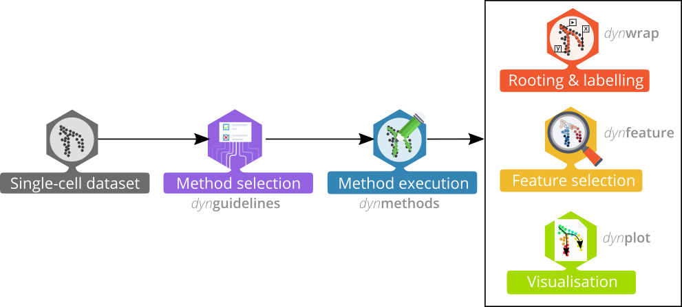
Preparing the data
The first step is to prepare the data for trajectory inference using wrap_expression. It requires both the counts and normalised expression (with genes/features in columns) as some TI methods are specifically built for one or the other:
data("fibroblast_reprogramming_treutlein")

dataset <- wrap_expression(
  counts = fibroblast_reprogramming_treutlein$counts,
  expression = fibroblast_reprogramming_treutlein$expression
)Selecting the best methods for a dataset
When the data is wrapped, the most performant and scalable set of tools can be selected using a shiny app. This app will select a set of methods which are predicted to produce the most optimal output given several user-dependent factors (such as prior expectations about the topology present in the data) and dataset-dependent factors (such as the size of the dataset). This app uses the benchmarking results from dynbenchmark (doi:10.1101/276907).
guidelines <- guidelines_shiny(dataset)
methods_selected <- guidelines$methods_selected
## Loading required namespace: akima
## [1] "slingshot" "paga_tree" "grandprix" "paga"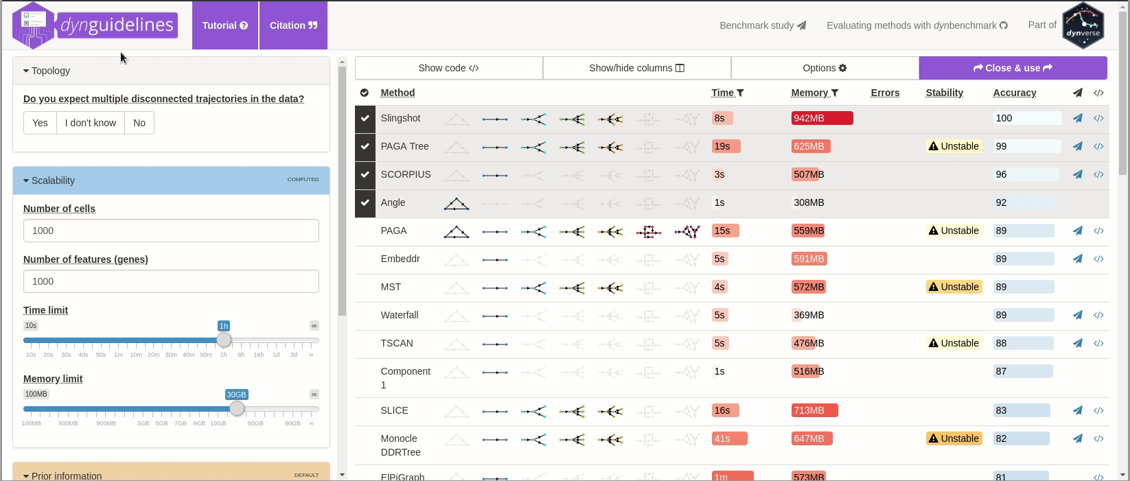
➽ An in-depth tutorial for selecting the most optimal set of methods
Running the methods
To run a method, it is currently necessary to have either docker or singularity installed. If that’s the case, running a method is a one-step-process. We will run the first selected method here:
model <- infer_trajectory(dataset, first(methods_selected))## Loading required namespace: hdf5rCurrently, the dynmethod package contains 59 methods!
Plotting the trajectory
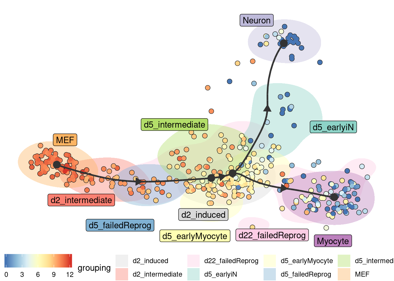
Several visualisation methods provide ways to biologically interpret trajectories.
Examples include combining a dimensionality reduction, a trajectory model and a cell clustering:
model <- model %>% add_dimred(dyndimred::dimred_mds, expression_source = dataset$expression)
plot_dimred(
  model,
  expression_source = dataset$expression,
  grouping = fibroblast_reprogramming_treutlein$grouping
)
## Coloring by grouping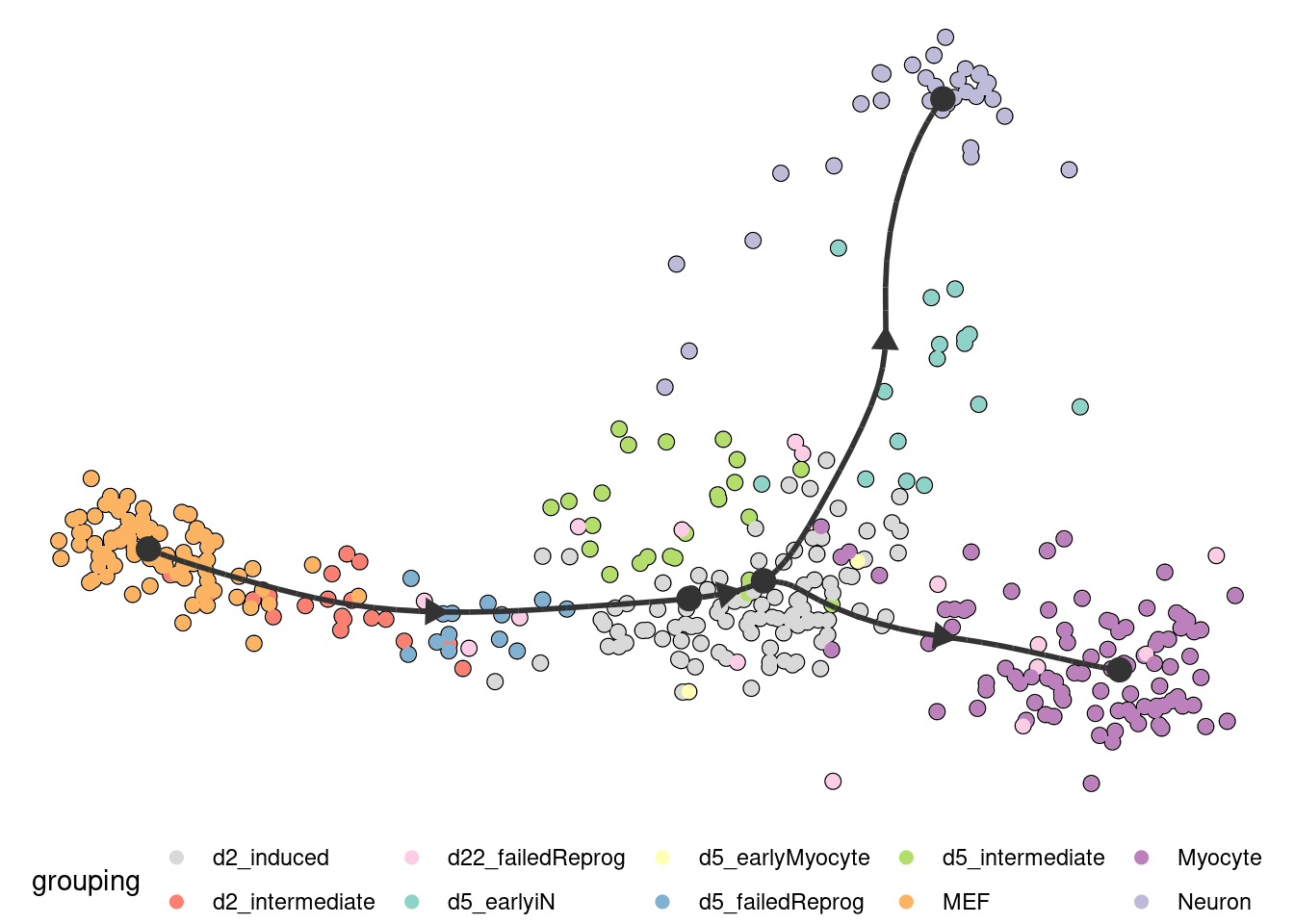
Similarly, the expression of a gene:
plot_dimred(
  model,
  expression_source = dataset$expression,
  feature_oi = "Fn1"
)
## Coloring by expression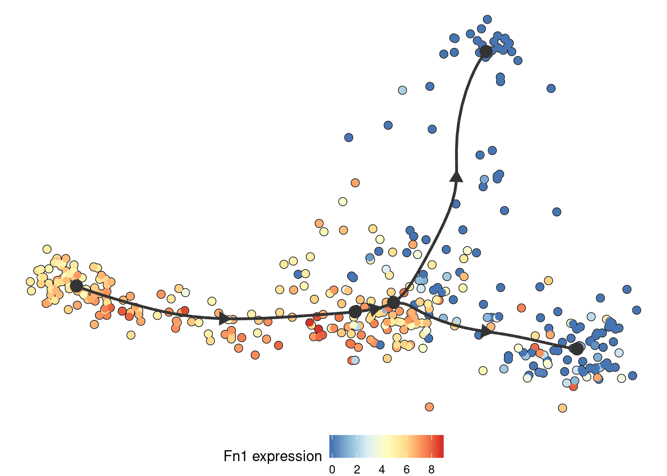
Groups can also be visualised using a background color
plot_dimred(
  model,
  expression_source = dataset$expression,
  color_cells = "feature",
  feature_oi = "Vim",
  color_density = "grouping",
  grouping = fibroblast_reprogramming_treutlein$grouping,
  label_milestones = FALSE
)
Interpreting the trajectory biologically
In most cases, some knowledge is present of the different start, end or intermediary states present in the data, and this can be used to adapt the trajectory so that it is easier to interpret.
Rooting
Most methods have no direct way of inferring the directionality of the trajectory. In this case, the trajectory should be “rooted” using some external information, for example by using a set of marker genes.
model <- model %>%
  add_root_using_expression(c("Vim"), dataset$expression)
Milestone labelling
Milestones can be labelled using marker genes. These labels can then be used for subsequent analyses and for visualisation.
model <- label_milestones_markers(
  model,
  markers = list(
    MEF = c("Vim"),
    Myocyte = c("Myl1"),
    Neuron = c("Stmn3")
  ),
  dataset$expression
)Predicting and visualising genes of interest
We integrate several methods to extract candidate marker genes/features from a trajectory.
A global overview of the most predictive genes
At default, the overall most important genes are calculated when plotting a heatmap.
plot_heatmap(
  model,
  expression_source = dataset$expression,
  grouping = fibroblast_reprogramming_treutlein$grouping,
  features_oi = 50
)
## No features of interest provided, selecting the top 50 features automatically
## Using dynfeature for selecting the top 50 features
## Coloring by grouping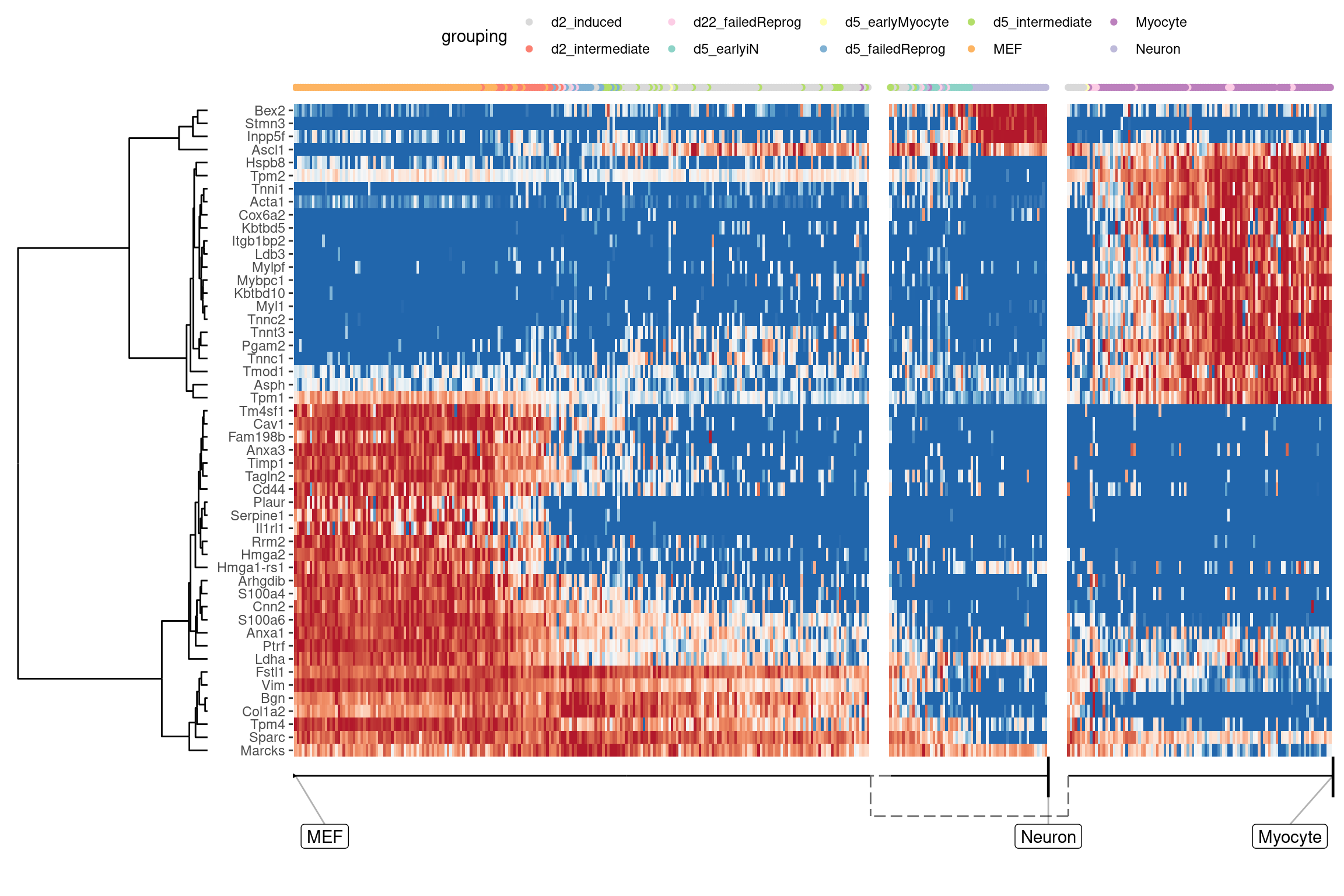
Lineage/branch markers
We can also extract features specific for a branch, eg. genes which change when a cell differentiates into a Neuron
branch_feature_importance <- calculate_branch_feature_importance(model, expression_source=dataset$expression)

neuron_features <- branch_feature_importance %>%
  filter(to == names(model$milestone_labelling)[which(model$milestone_labelling =="Neuron")]) %>%
  top_n(50, importance) %>%
  pull(feature_id)
plot_heatmap(
model,
expression_source = dataset$expression,
features_oi = neuron_features
)
## Coloring by milestone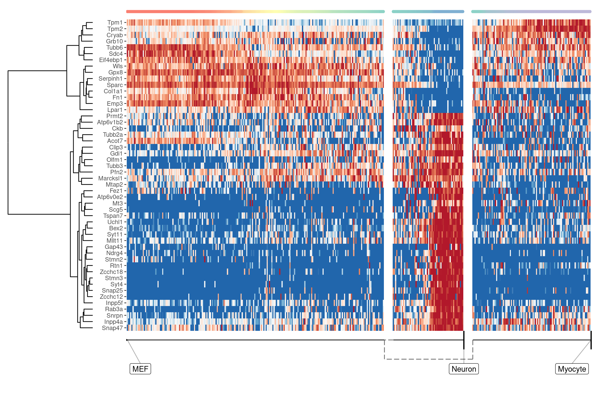
Genes important at bifurcation points
We can also extract features which change at the branching point
branching_milestone <- model$milestone_network %>% group_by(from) %>% filter(n() > 1) %>% pull(from) %>% first()

branch_feature_importance <- calculate_branching_point_feature_importance(model, expression_source=dataset$expression, milestones_oi = branching_milestone)

branching_point_features <- branch_feature_importance %>% top_n(20, importance) %>% pull(feature_id)

plot_heatmap(
  model,
  expression_source = dataset$expression,
  features_oi = branching_point_features
)
## Coloring by milestone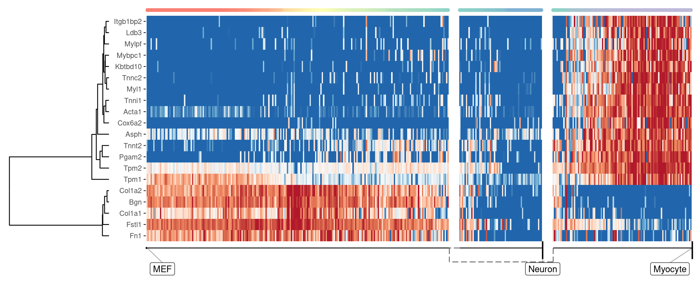
space <- dyndimred::dimred_mds(dataset$expression)

map(branching_point_features[1:12], function(feature_oi) {
  plot_dimred(model, dimred = space, expression_source = dataset$expression, feature_oi = feature_oi, label_milestones = FALSE) +
    theme(legend.position = "none") +
    ggtitle(feature_oi)
}) %>% patchwork::wrap_plots()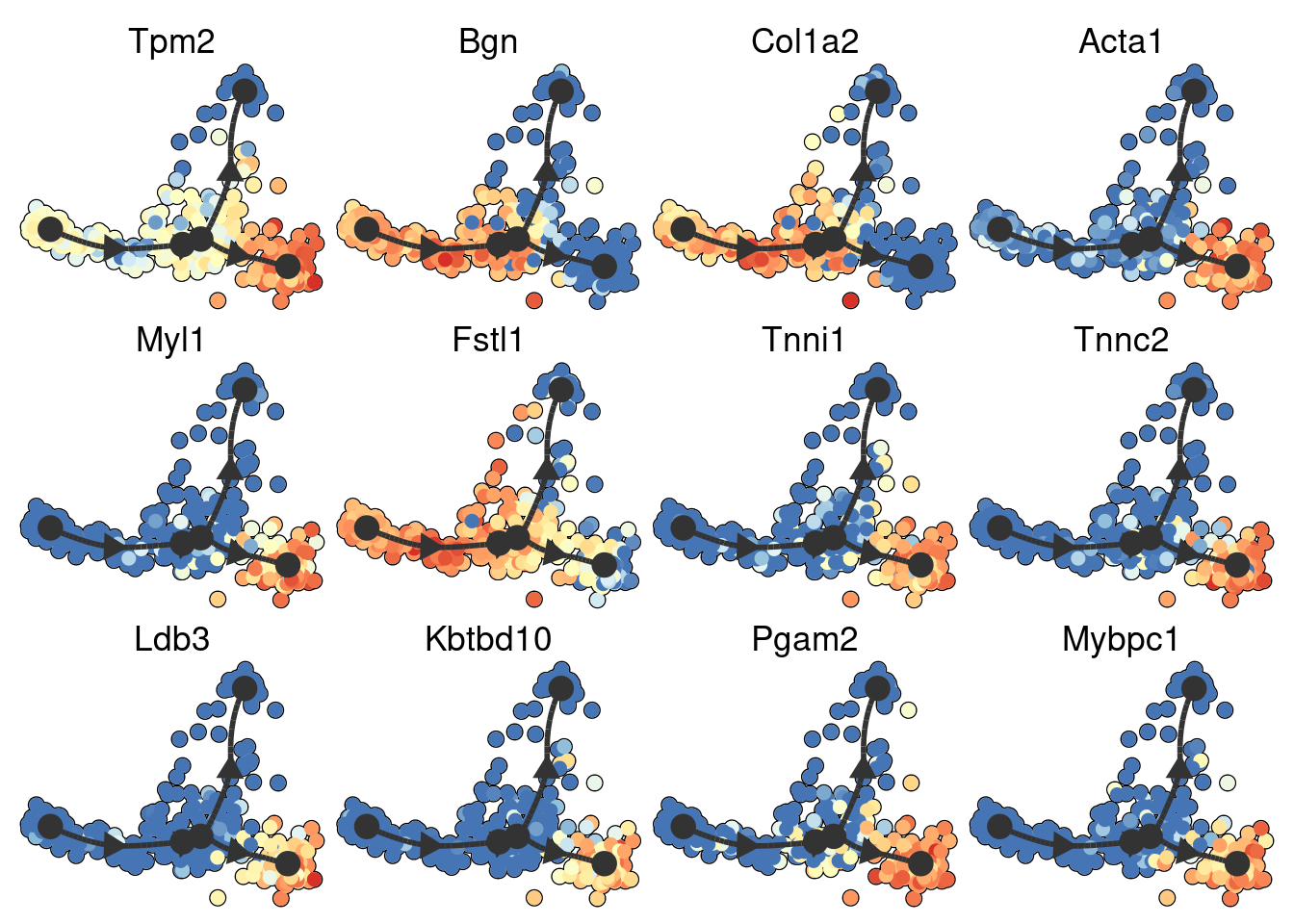
➽ An in-depth tutorial for finding trajectory differentially expressed genes